I experimented with 4 metrics:
The broad approach was to exhaustively search about a [-15, 15] interval for different alignments of the green and red channel to the blue channel. For each offset, we calculate the metric and we pick the "best" one. In practice, I negated the NCC so that this meant picking the offset that minimizes the metric of choice.I thought of using normalized L2 distance to compensate for brightness differences, and L1 distance because it might be more robust to outliers, but experimentally, this did not hold. The alignments were being thrown off due to the edges of the picture needlessly adding to the score, so I introduced a parameter k that specified what margins to disregard when computing the metric. I played around with k=5, 10, 20 and noticed that the outputs could be slightly sensitive to that factor. Note that both NCC and L2 Distance gave similar outputs, I picked L2 Distance for the following example with the cathedral. Note how k=20 performs best, but k=10 performs worse than when k=5. Future steps could incorporate automatic cropping or hyperparameter tuning to pick the best value of k. My function does also support float values of k between 0 and 1 (percentages of height or width), but I felt the hardcoded values were clearer to me. For the higher resolution images, this would have a marginal effect even with the multiscale approach described in the next section.
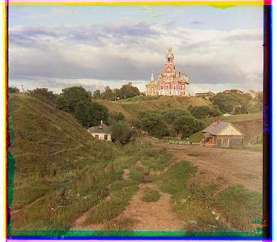
NCC, k=20,
R->G = (1, 7),
B->G = (-2, -5)
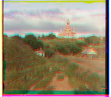
NCC, k=10,
R->G = (1, 0),
B->G = (-2, -5)
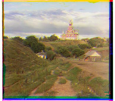
NCC, k=5,
R->G = (0, 6),
B->G = (1, -7)
Other pictures also turned out quite fine with the same parameters, below I show tobolsk, monastery with the default parameter I found, k=5. I also found that L2 Distance was more sensitive to the choice of k, hence I opted to use NCC in the below cases, even though both provided the same outputs on these specific images:
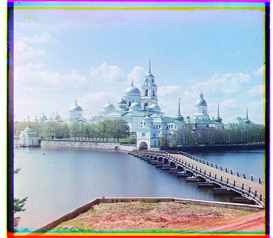
NCC, k=5,
R->B = (2, 3),
G->B = (2, -3)
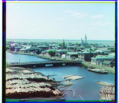
NCC, k=5,
R->B = (3, 6),
G->B = (2, 3)
Multiscale Scale Images
With higher-resolution images, the same exhaustive search took too long. This called for the use of a pyramid scheme (not the scam). Effectively, the logic goes: downsample the image (while avoiding aliasing) till it is small enough to do a naive search, then go up to progressively higher resolutions, using a smaller [-2, 2] interval search to gradually mak finer-grained movements towards a reasonable offset. My pseudocode looked like:
def align_multiscale(im1, im2, depth):

	if depth is 0:

		find_best_offset(im1, im2, [-15, 15] search space)

	else:

		rescale im1 and im2 by 0.5, ensure anti-aliasing is on

		x, y = align_multiscale(im1_rescaled, im2_rescaled, depth-1)

		dx, dy = find_best_offset(im1, translated(im2, dx, dy), [-2, 2] search space)

		return 2*x + dx, 2*y+dy
Generally I found a lot more success here. As opposed to aligning the .tif images on the order of minutes, within 15 seconds I got well-aligned images. Some examples below:

L2 Distance, k=5,
R->B = (12, 112),
G->B = (9, 50)

L2 Distance, k=5,
R->B = (14, 124),
G->B = (17, 60)
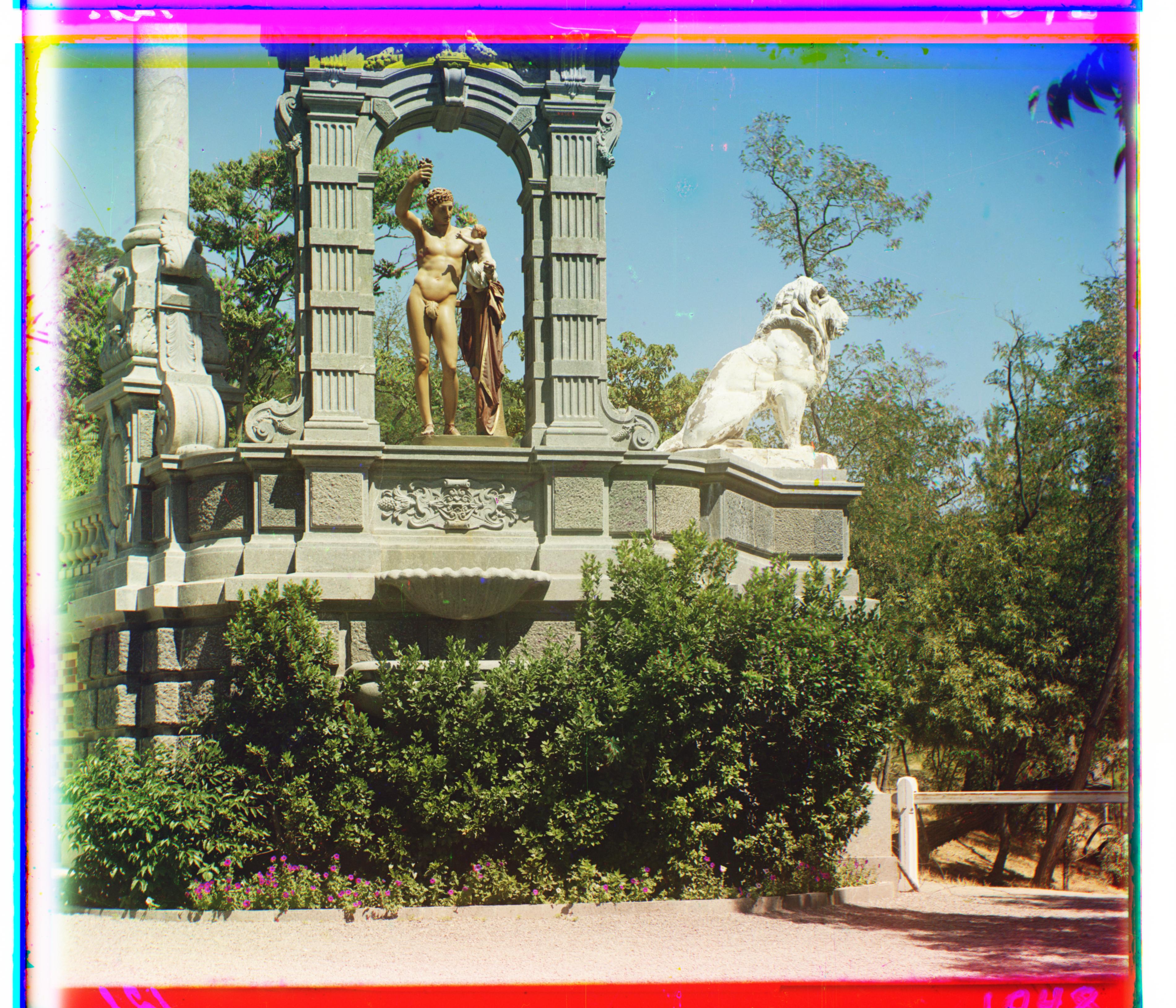
L2 Distance, k=5,
R->B = (-27, 140),
G->B = (-11, 33)
L2 Distance, k=5,
R->B = (23, 90),
G->B = (17, 41)

L2 Distance, k=5,
R->B = (-4, 58),
G->B = (4, 25)
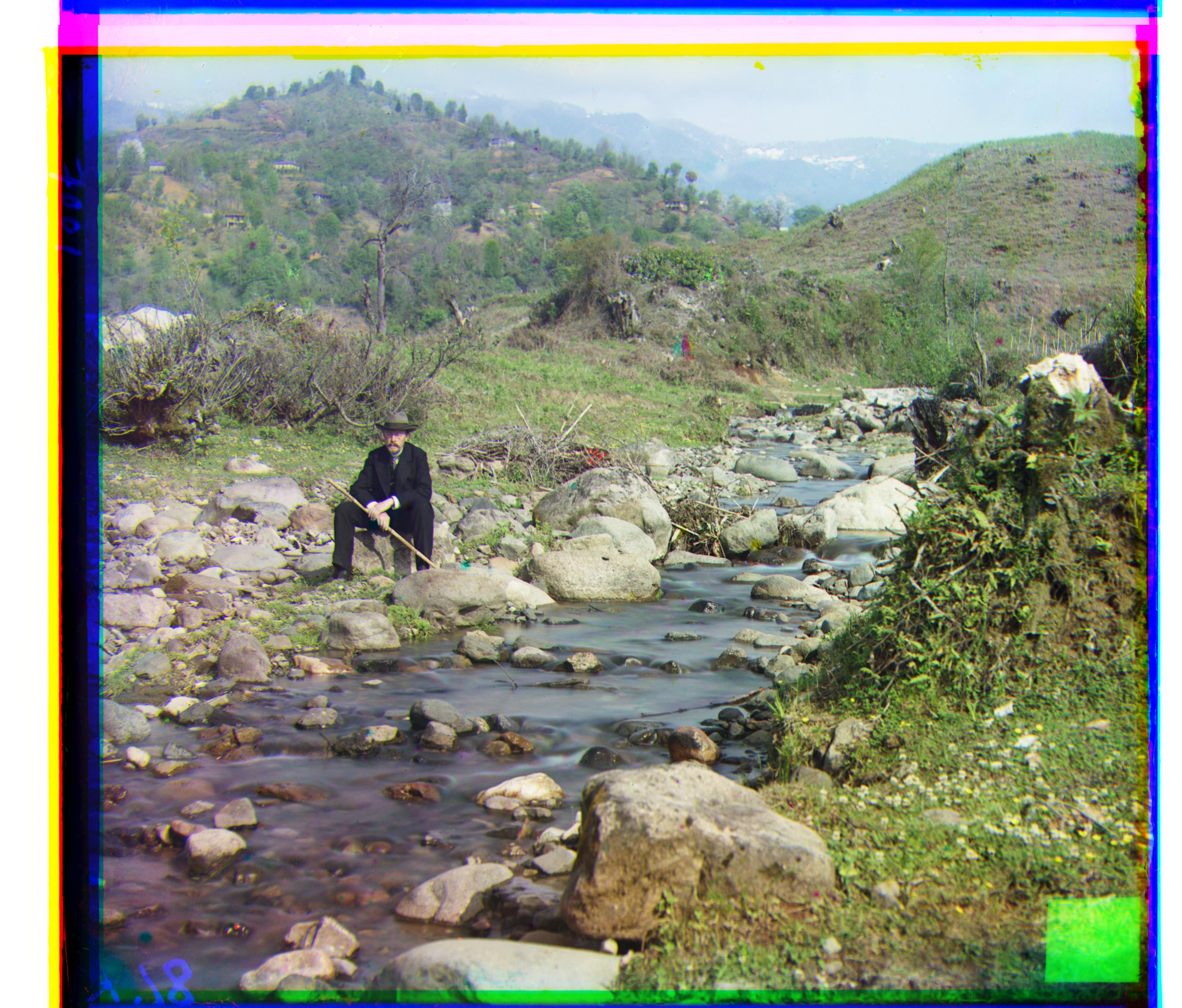
L2 Distance, k=5,
R->B = (37, 176),
G->B = (30, 80)
The emir proved to be more difficult, largely due to the stark differences in brightness between the red filter and the other two filters. I found this effect was particularly emphasised with L2 distance. Instead of aligning red and green to blue, I found success in aligning red and blue to green instead. I did also have to tune the margin-cropping parameter k more to achieve this outcome. While I dabbled with Canny edge detection, the tradeoff in terms of time didn't seem proportional for generally equivalent results to the green-aligned version.
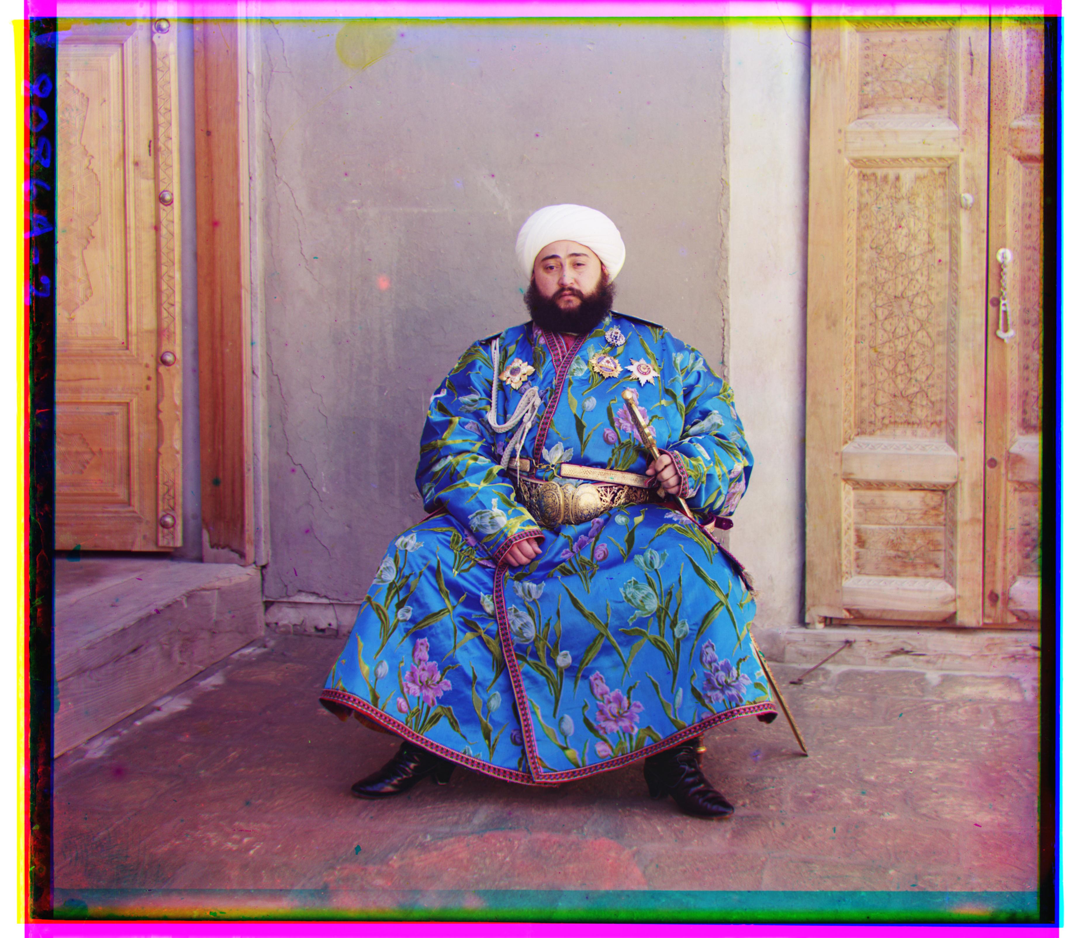
L2 Distance, k=5,
R->G = (17, 57),
G->B = (-24, 49)
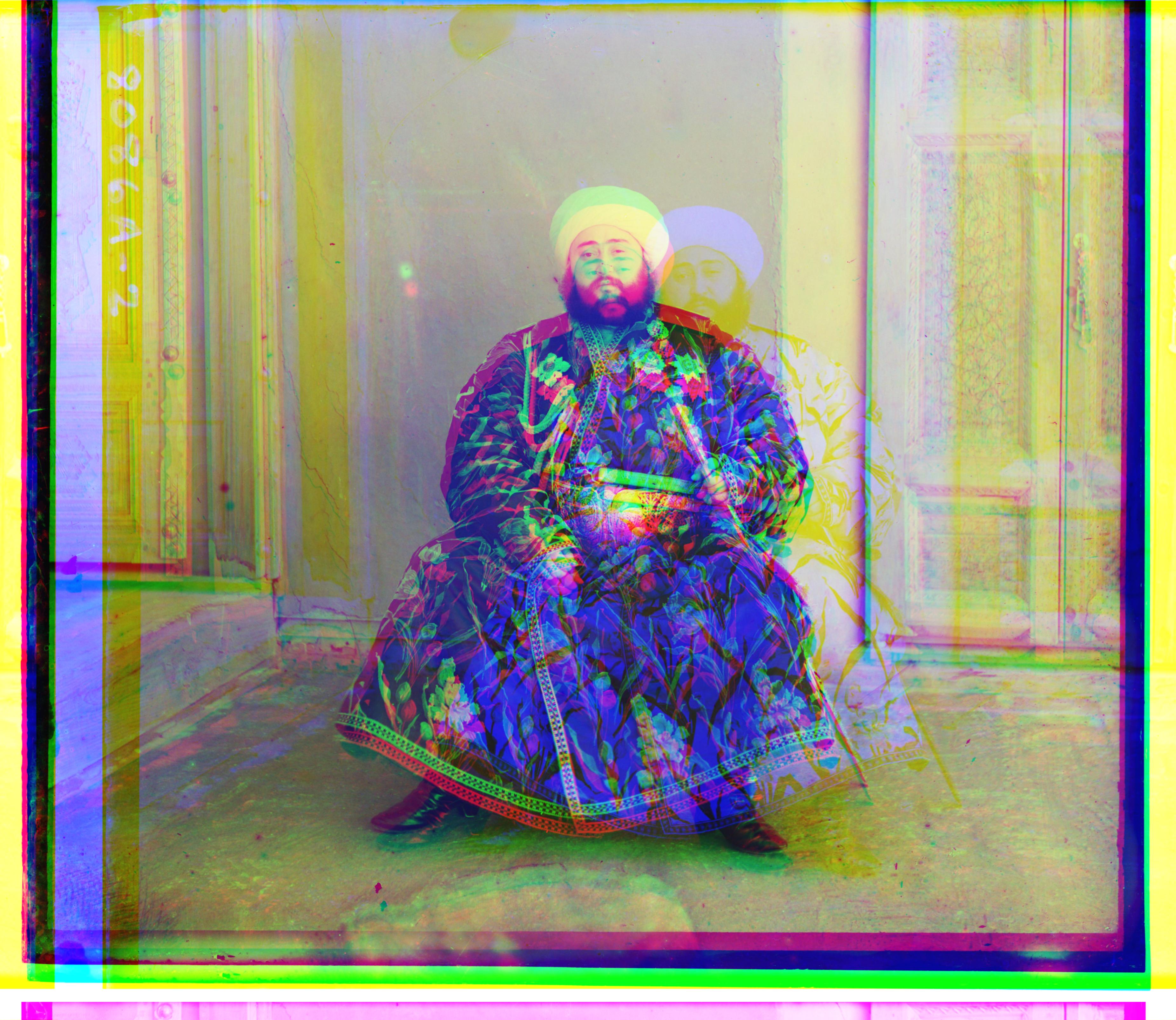
L2 Distance, k=5,
G->R = (-17, -57),
G->B = (523,-158)
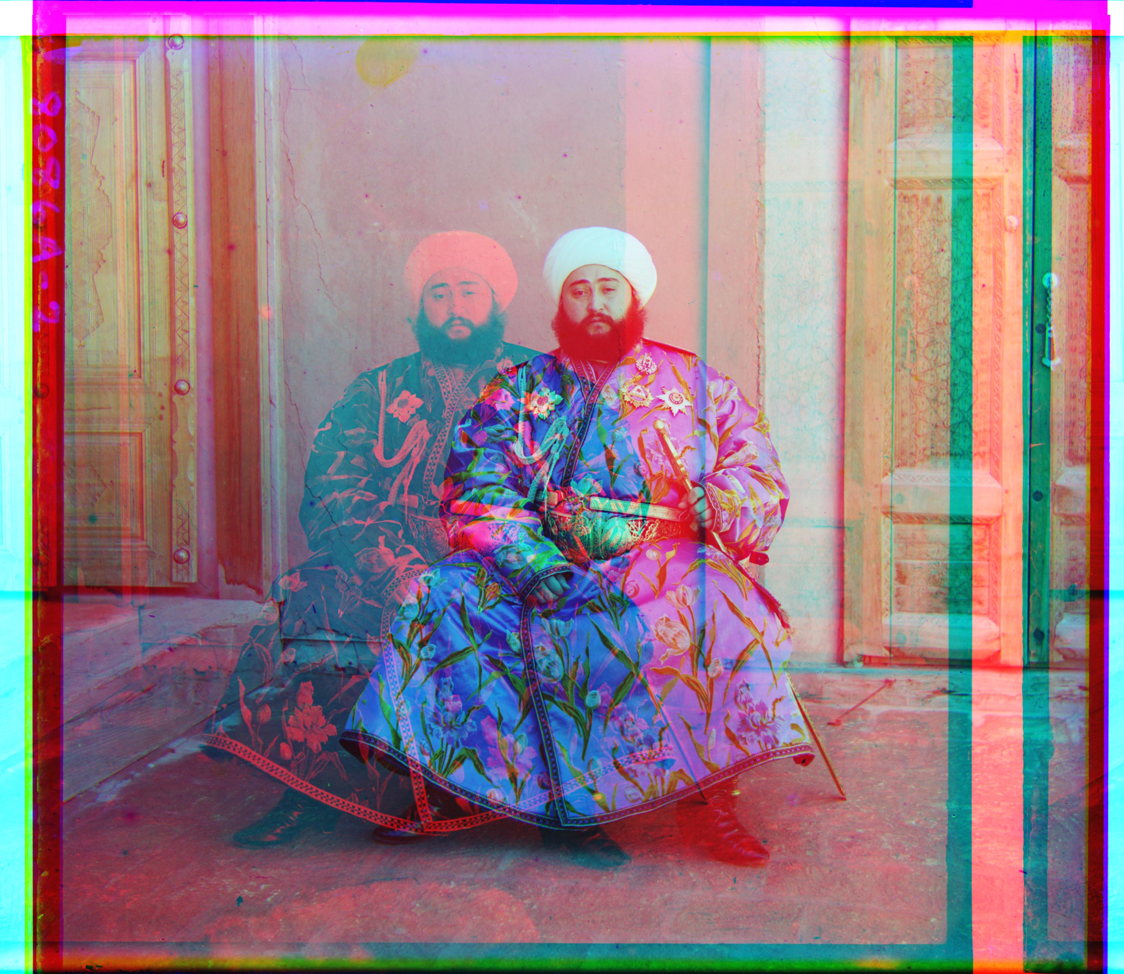
L2 Distance, k=5,
R->B = (-418, 118),
G->B = (24, 49)
Multiscale Scale Images
With higher-resolution images, the same exhaustive search took too long. This called for the use of a pyramid scheme (not the scam). Effectively, the logic goes: downsample the image (while avoiding aliasing) till it is small enough to do a naive search, then go up to progressively higher resolutions, using a smaller [-2, 2] interval search to gradually mak finer-grained movements towards a reasonable offset. My pseudocode looked like:
def align_multiscale(im1, im2, depth):

	if depth is 0:

		find_best_offset(im1, im2, [-15, 15] search space)

	else:

		rescale im1 and im2 by 0.5, ensure anti-aliasing is on

		x, y = align_multiscale(im1_rescaled, im2_rescaled, depth-1)

		dx, dy = find_best_offset(im1, translated(im2, dx, dy), [-2, 2] search space)

		return 2*x + dx, 2*y+dy
Generally I found a lot more success here. As opposed to aligning the .tif images on the order of minutes, within 15 seconds I got well-aligned images. Some examples below:

L2 Distance, k=5,
R->B = (12, 112),
G->B = (9, 50)

L2 Distance, k=5,
R->B = (14, 124),
G->B = (17, 60)

L2 Distance, k=5,
R->B = (-27, 140),
G->B = (-11, 33)
L2 Distance, k=5,
R->B = (23, 90),
G->B = (17, 41)

L2 Distance, k=5,
R->B = (-4, 58),
G->B = (4, 25)

L2 Distance, k=5,
R->B = (37, 176),
G->B = (30, 80)
The emir proved to be more difficult, largely due to the stark differences in brightness between the red filter and the other two filters. I found this effect was particularly emphasised with L2 distance. Instead of aligning red and green to blue, I found success in aligning red and blue to green instead. I did also have to tune the margin-cropping parameter k more to achieve this outcome. While I dabbled with Canny edge detection, the tradeoff in terms of time didn't seem proportional for generally equivalent results to the green-aligned version.

L2 Distance, k=5,
R->G = (17, 57),
G->B = (-24, 49)

L2 Distance, k=5,
G->R = (-17, -57),
G->B = (523,-158)

L2 Distance, k=5,
R->B = (-418, 118),
G->B = (24, 49)
Bells and Whistles: Phase Correlation
Exhaustive searching takes time and is overly reliant on pixel values. In practice, experimenting and tuning the margins, the range to search over, which channel to align to all takes time. We don't want to take time. Enter phase correlation. I came across it in the textbook, and Wikipedia provided a formula. The premise is, let's move from the time domain to frequency domain using a 2D fourier transform, compute the cross-correlation there very efficiently, and then move back into the time domain using a 2D inverse FFT and find the offset which maximizes the cross-correlation. It's beautiful, and much faster than anything above, especially given that it's performing a global search (not just over the interval specified).
It worked wonders for both the jpgs and tifs, including the infamous emir. Note that the really large offsets are a consequence of the fact that it returns x, y that are positive. In a image that is 3900 pixels wide, a shift 3800 to the right is the same as -100. This also proved to be useful for visual debugging, especially when working with the cathedral and emir images. For example, I could glean that the Green to Blue shift was fine in the case of the emir since both my pyramid and phase correlation method got (24, 49), but the red to blue shifts were very different.
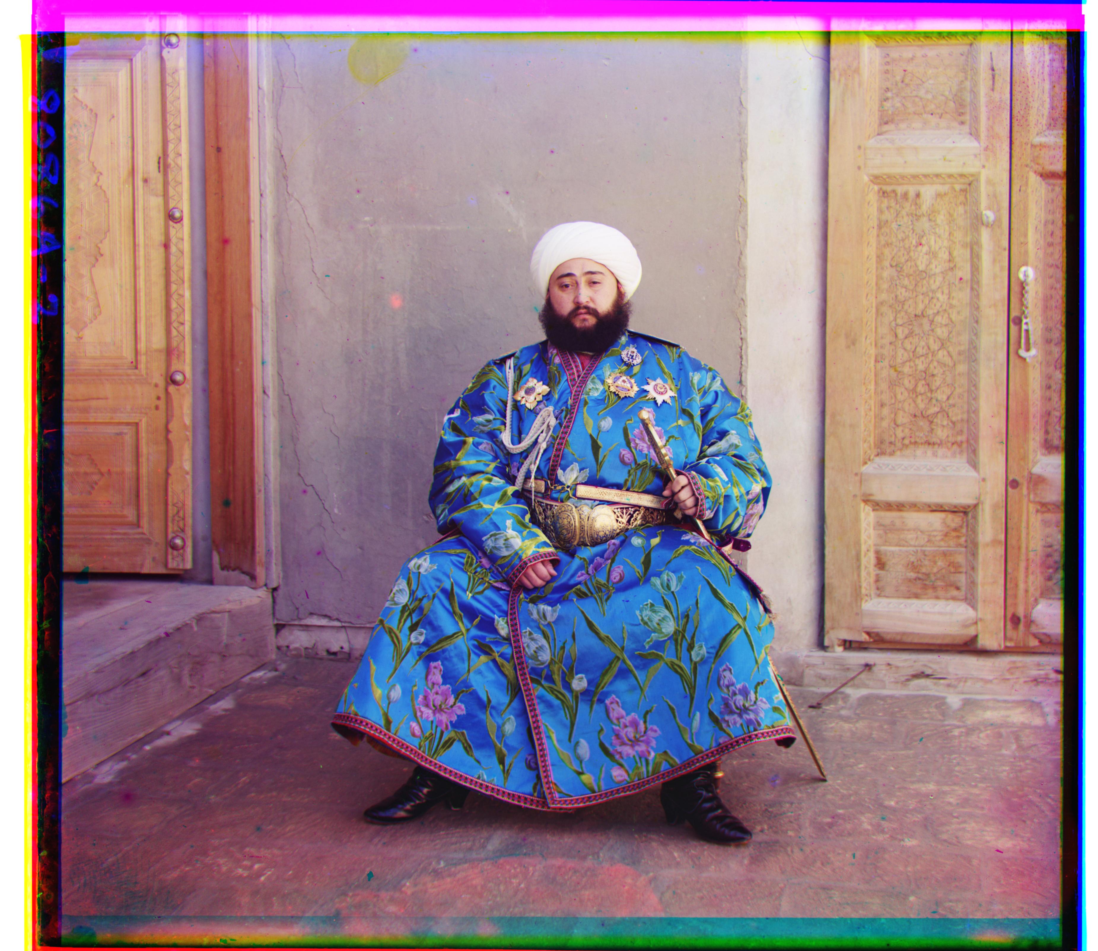
NCC
R->B = (41, 106),
G->B = (24, 49)
NCC
R->B = (3, 12),
G->B = (2, 5)
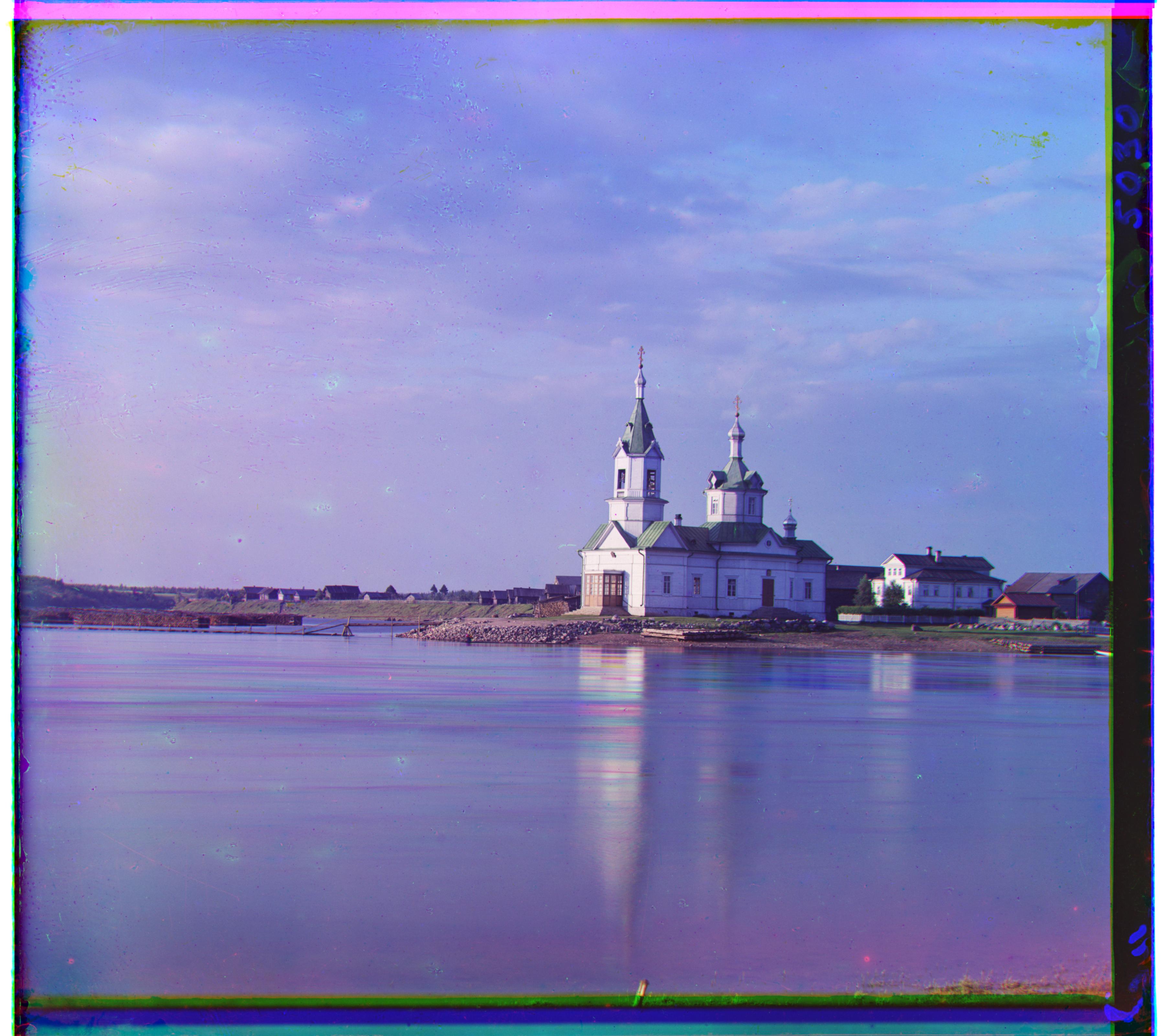
NCC
R->B = (3630, 58),
G->B = (3, 25)
NCC
R->B = (23, 88),
G->B = (16, 39)

NCC
R->B = (3773, 140),
G->B = (3789, 33)
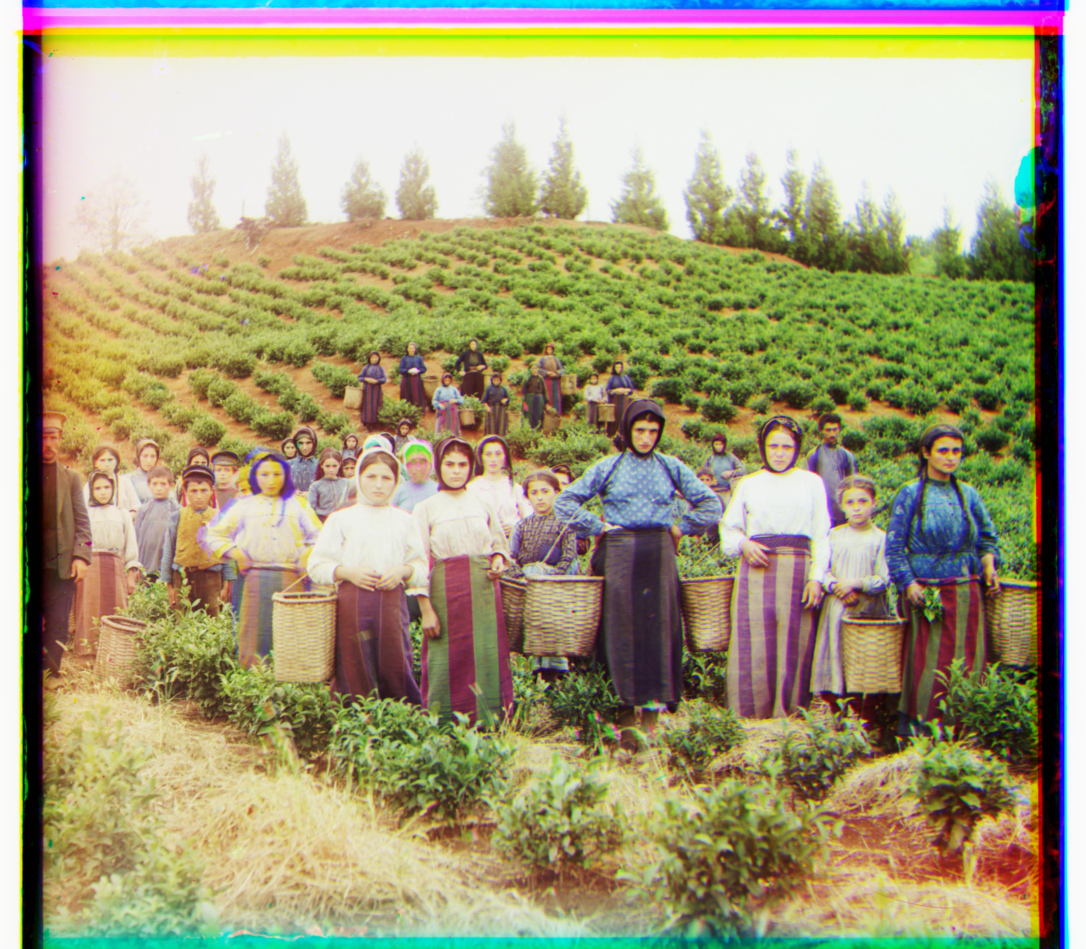
NCC
R->B = (11, 118),
G->B = (11, 55)

NCC
R->B = (37, 175),
G->B = (29, 77)
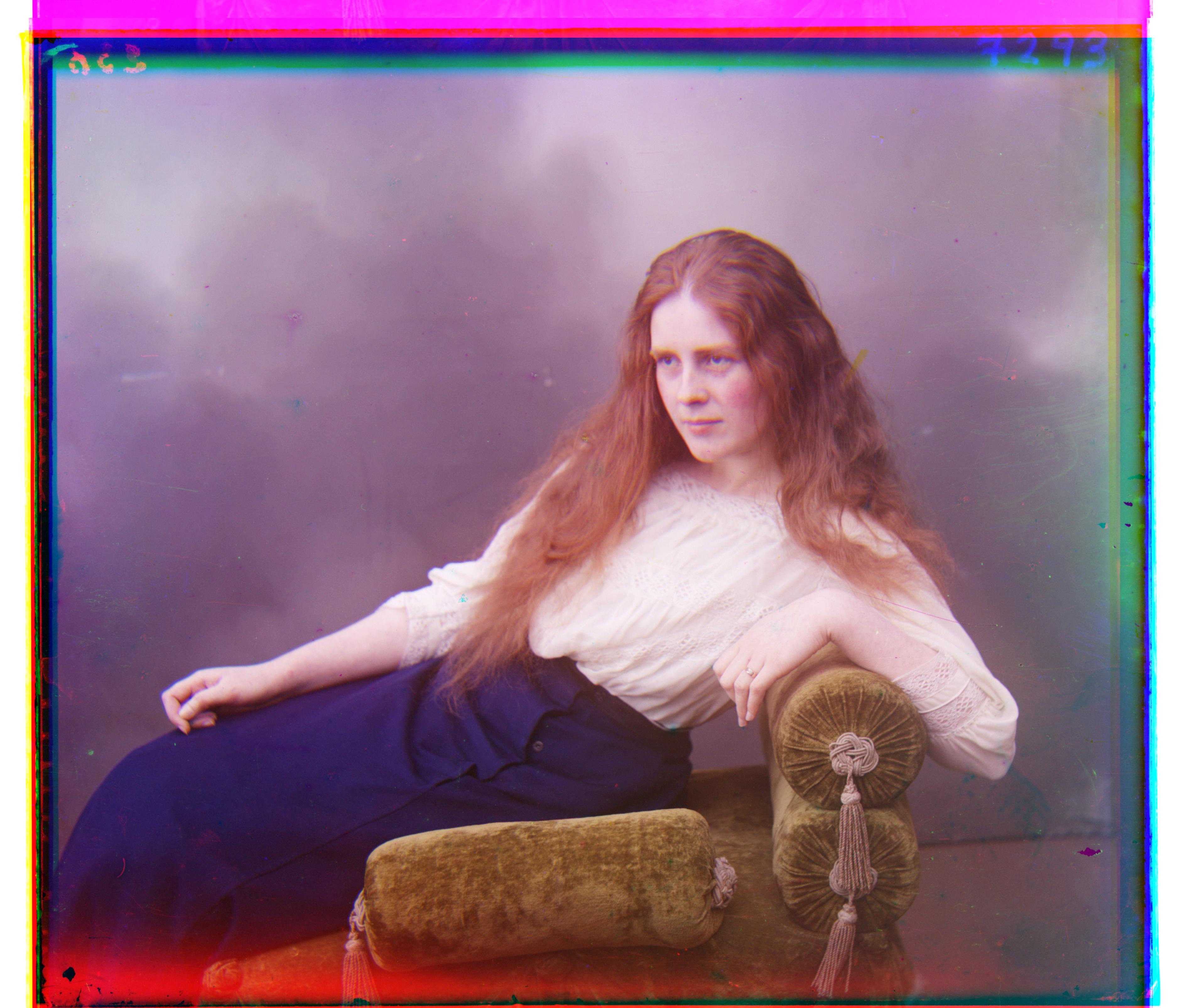
NCC
R->B = (13, 120),
G->B = (9, 57)
Bells and Whistles: Custom Images
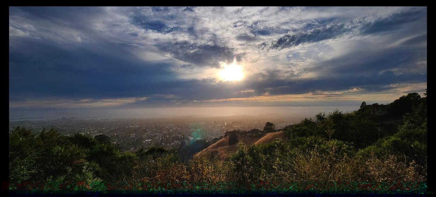
These pictures are old. Pretty cool, but old. I wanted to see separate pictures I had taken, and then use my algorithm to align them again. So I took my own LinkedIn picture and a sunset picture I had taken from the fire trails, tinkered with photoshop and aligned them using the multiscale and phase correlation approaches.
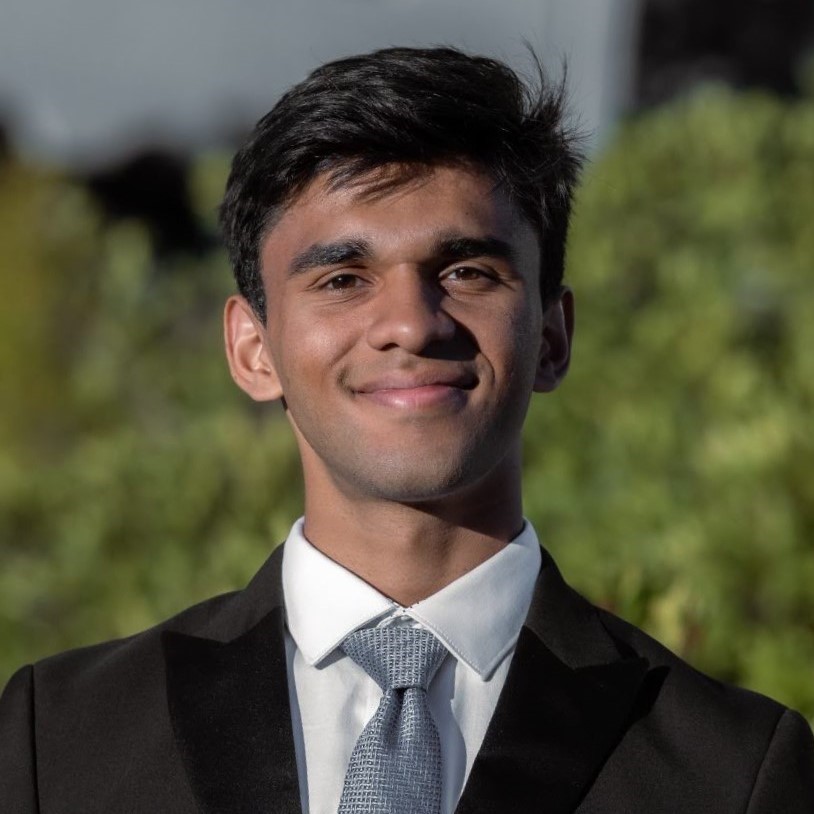
Original Image
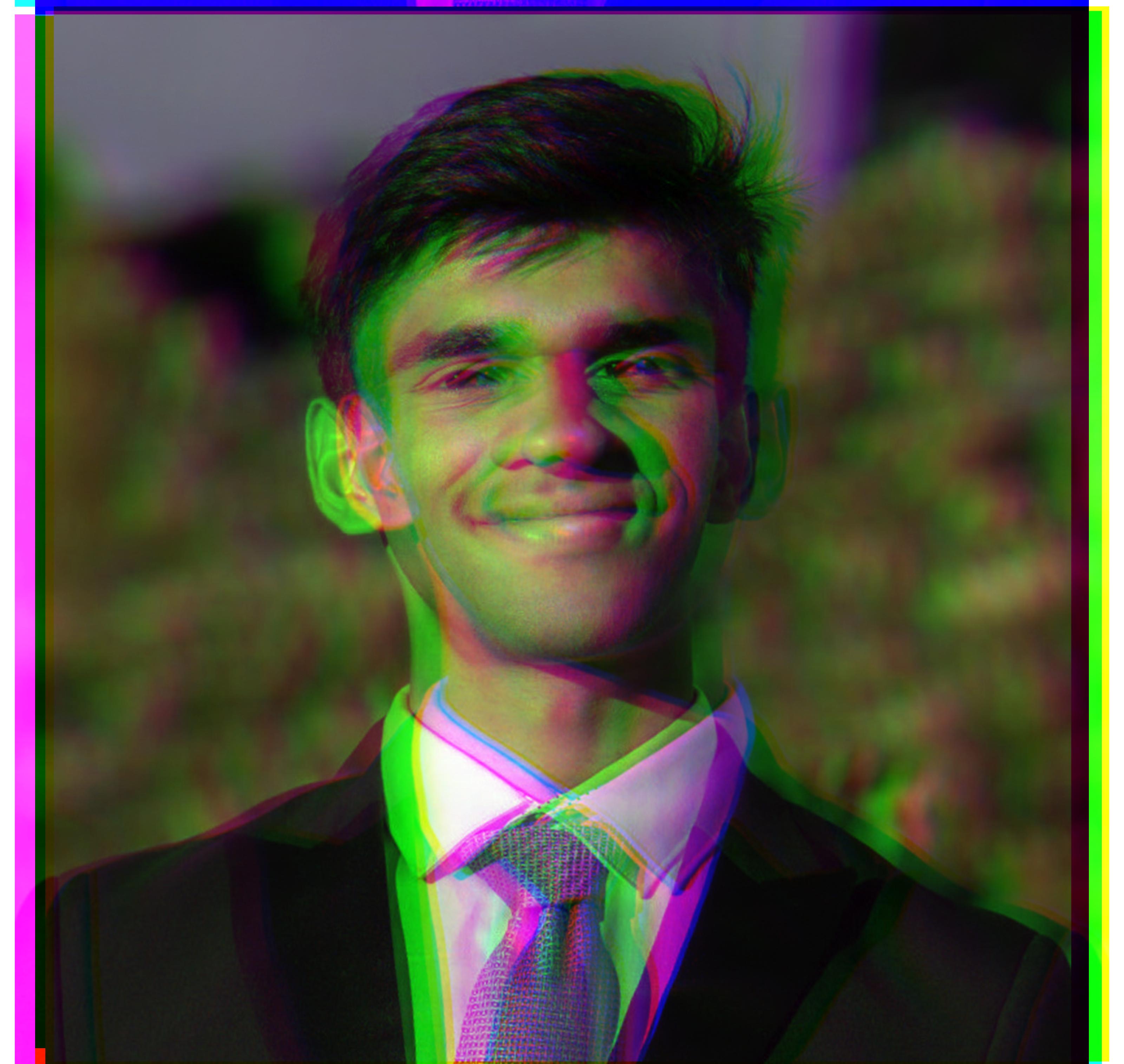
Unaligned
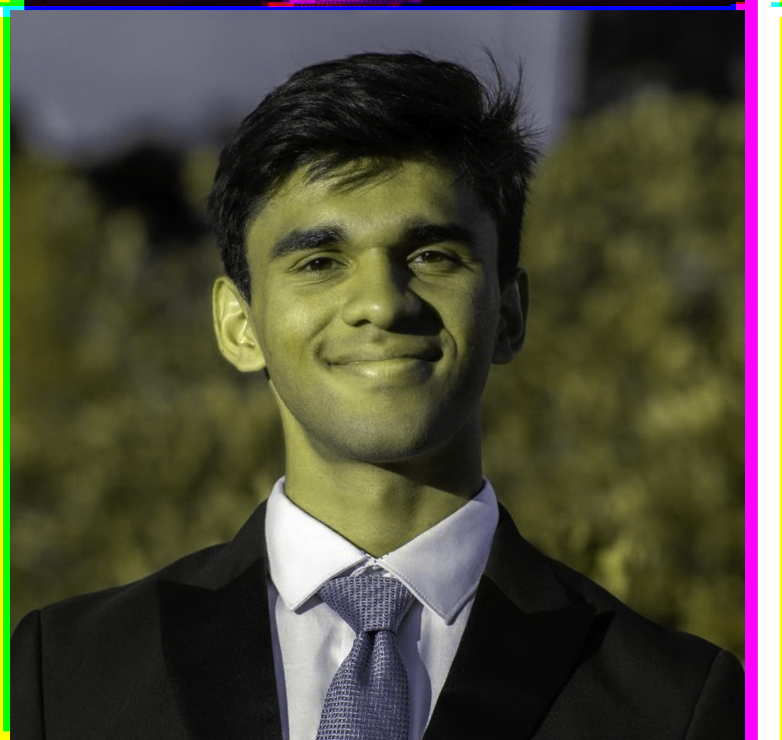
L2 Distance
R->B = (23, -14),
G->B = (110, -24)
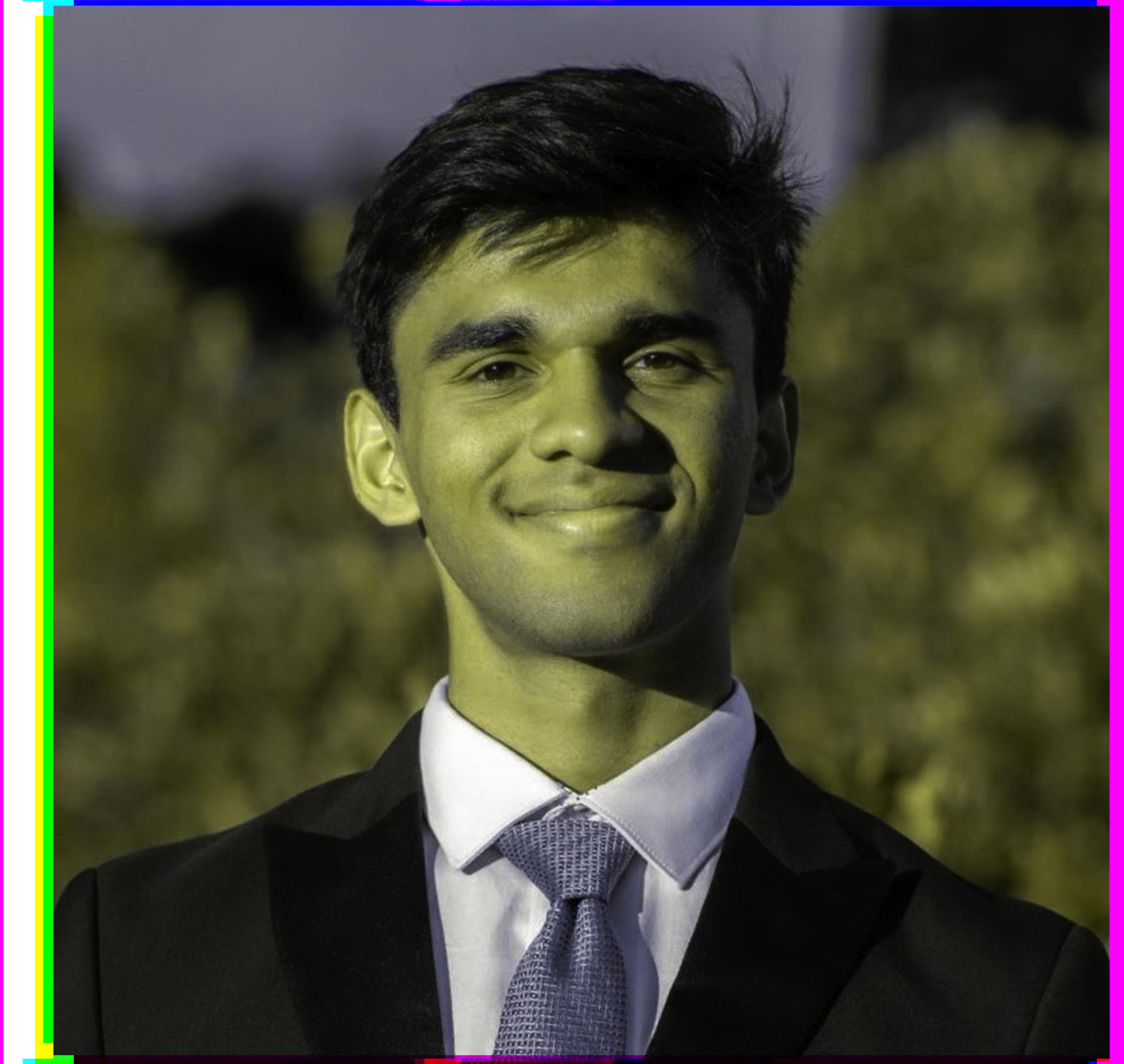
Phase Correlation, NCC
R->B = (3630, 58),
G->B = (3, 25)
Why I suddenly turned yellow is a mystery in its own right, but the outcome was still pretty satisfying. I think it has to do with how the frames are being stacked up. With more time, I would have investigated the orange and yellow filters that Photoshop also allows you to extract, which I didn't include as skio did not support 5-channel images. For the sunset,
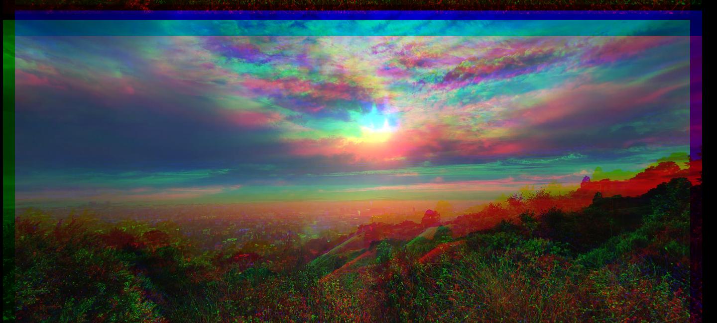
Unaligned
L2 Distance
R->B = (0, 599),
G->B = (24, 631)
Sunset feels like the perfect way to close out a pretty fun project overall!