In Project 4A, I took a bunch of pictures, recovered homographies, warped images and then blended them together to form mosaics and panoramas.
CS 180 Project: Image Mosaics
Part A & B
Table of Contents
Part A
Part B
Part 1. Introduction
Part 2: Computing Homographies and Warping
The compute_homography function calculates the homography matrix between two sets of
corresponding points. The function takes two input arrays: points from the first image and corresponding points in the target image.
It constructs a system of linear equations and solves them using the least squares method to find the optimal homography
matrix.
The warp_image function applies the computed homography to warp an input image. It uses the inverse of the homography matrix to map coordinates from the output image back to the input image. The function then uses bilinear interpolation to sample pixel values from the input image, ensuring smooth transitions between pixels in the warped result.
Part 3: Image Rectification
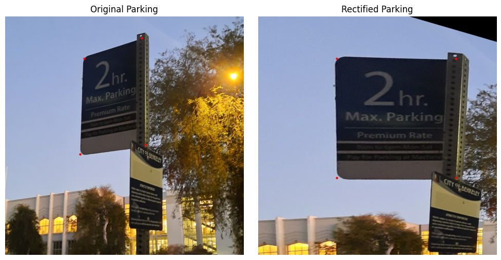
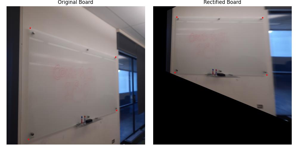
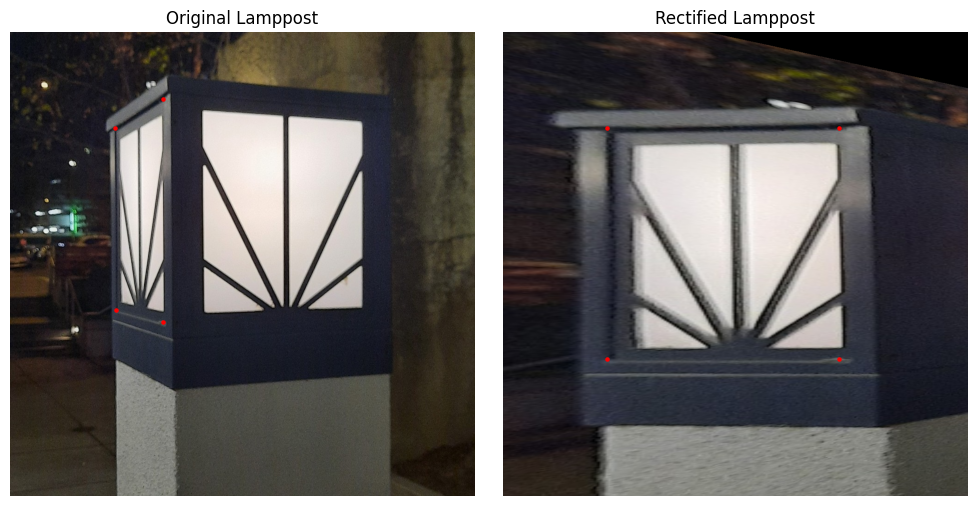
I picked an assortment of things to rectify: a parking sign near my apartment, the whiteboard in Evans 1015 (ft. CS 180) and a lamppost. You can see the correspondence points I picked marked in red. I was particularly happy with the rectification of the lamppost given how small the region was. For the board, I drew out COMPSCI 180 in bubble letters to also verify that the transformation preserved text written on the same plane as the changes.
Part 4: Mosaics
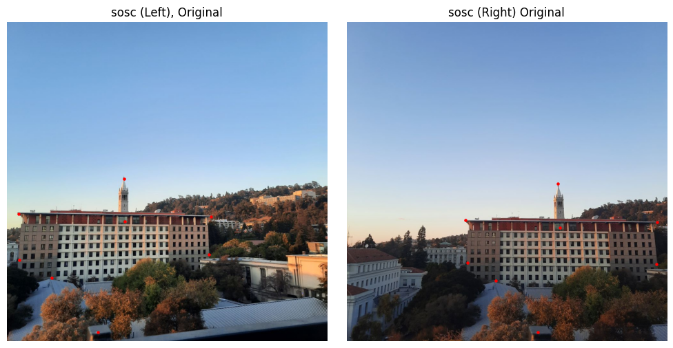
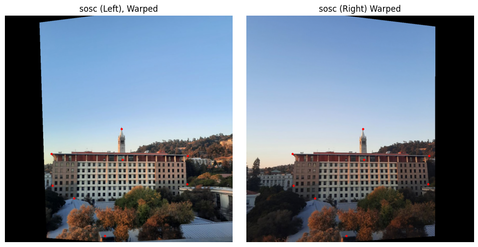
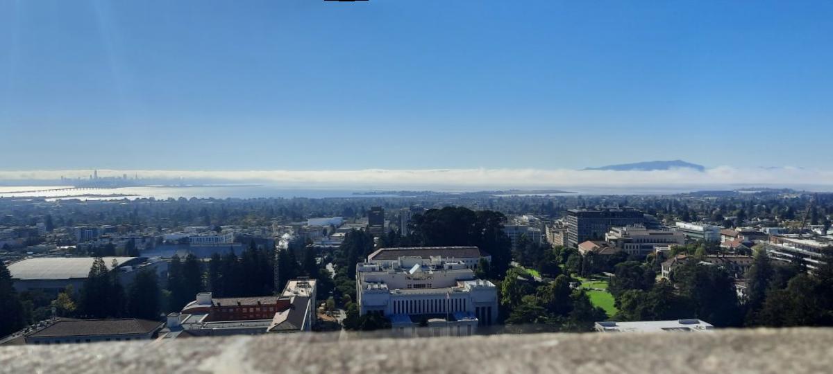
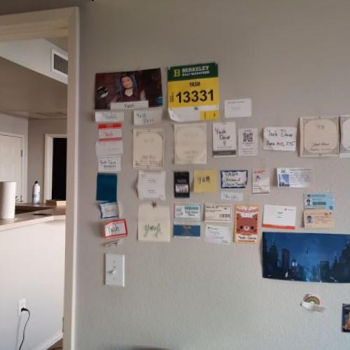
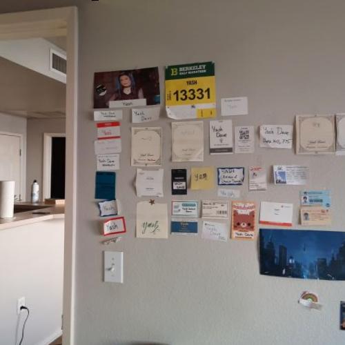
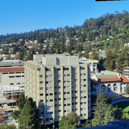
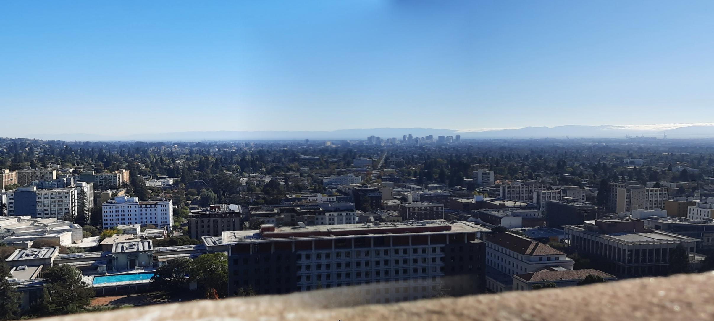
I am a fan of landscapes so a lot of my mosaics stem from pictures I took from the Campanile (Northside, Bayview) and at the rooftop of the Standard (sosc, short for Social Sciences Bldg). In addition, and for some variety, I also took a couple of pictures of my room and stitched them together to show that the process works for nearby objects as well.
My approach was:
- Use the correspondence tool from Project 3 to match features in two images
- Compute the midway points using them (
center_pts) - Project each image onto the midway points
- Create two masks using both
left_warpedandright_warped - Apply cv2.distanceTransform to get more gradual masks and prevent sharp lines
- Perform a weighted sum using these masks and normalize accordingly to get the combined image
I included a naive combination of the two warped images by just taking an average as well. Some of the high filter features (like text in the wall picture) appear slightly blurry as they don't precisely line up with their opposing counterparts. I fiddled around with laplacian pyramids and sharpening but, in my opinion, it made the pictures worse. I attributed this to the warping step, wherein some pixels would necessarily get distributed across others when doing the bilinear interpolation. This is particularly pronounced for wide-angle shots (like Bayview), and was unlikely to be fixed by emphasizing the high filter components.
SOSC Mosaic
For this first mosaic, I also included the left and right masks I obtained for each image.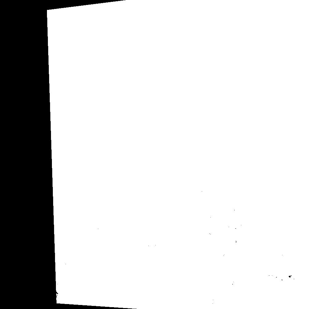
SOSC: Left Mask
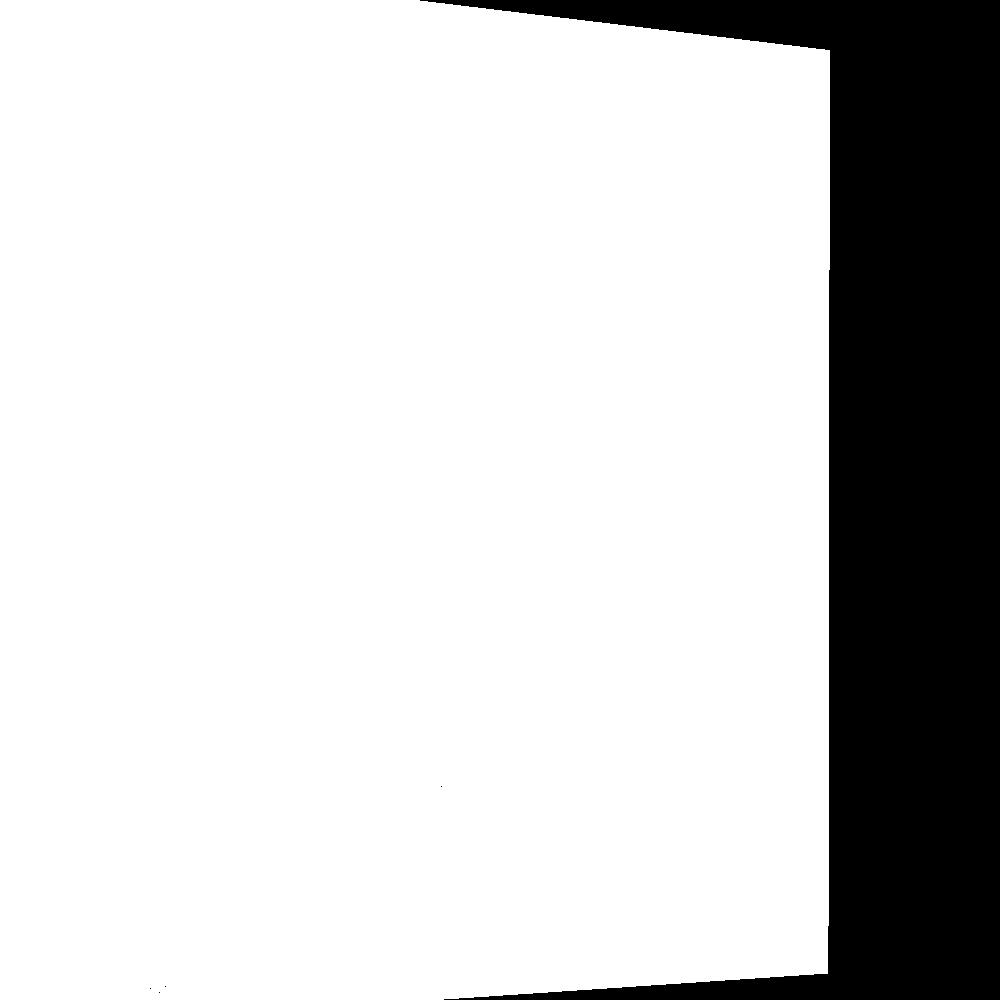
SOSC: Right Mask
SOSC: Distance Transform Masks
SOSC: Warped Images
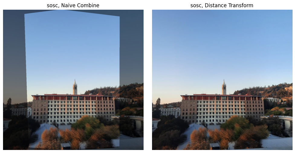
SOSC: Naive Combine and Distance Transform
Northside Mosaic

Northside: Original Images with Points
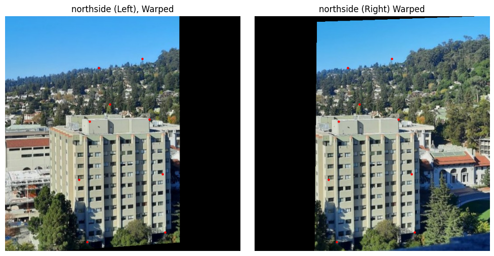
Northside: Warped Images
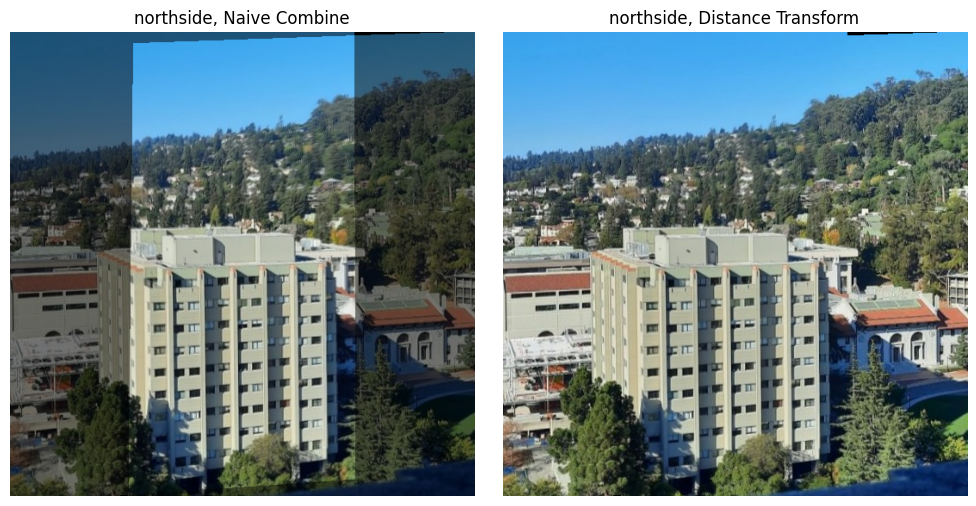
Northside: Naive Combine and Distance Transform
Bayview Mosaic

Bayview: Original Images with Points

Bayview: Warped Images
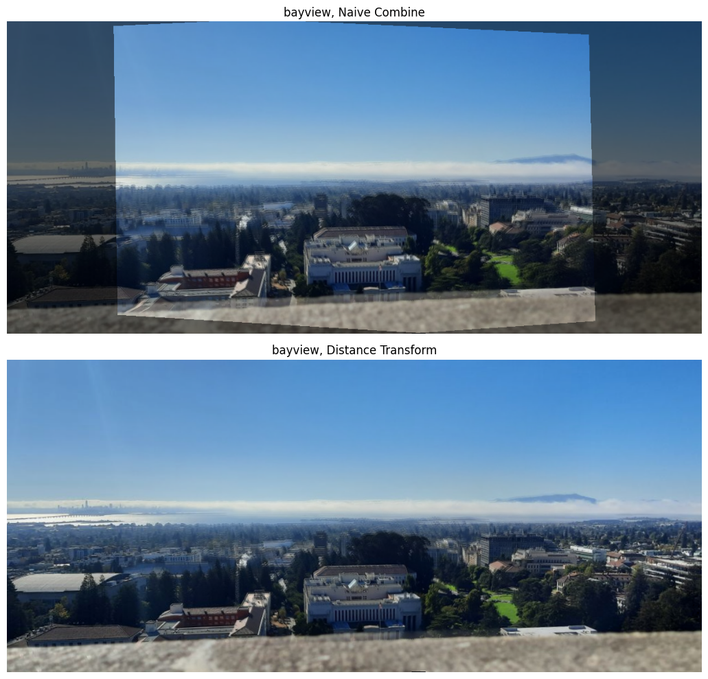
Bayview: Naive Combine and Distance Transform
Wall Mosaic
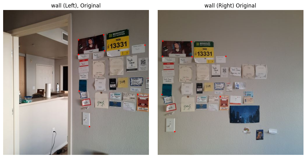
Wall: Original Images with Points
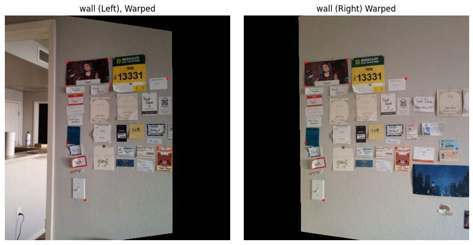
Wall: Warped Images
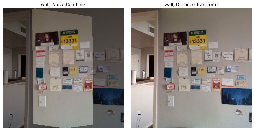
Wall: Naive Combine and Distance Transform
Part B
Detecting Corners
In my implementation, I began by detecting corners using the Harris algorithm through get_harris_corners(). After extracting the corner scores into a vector using scores = h[corners[:, 0], corners[:, 1]], I moved on to applying Adaptive Non-Maximal Suppression (ANMS). This crucial step helps me identify the strongest corners while ensuring they remain evenly distributed across the image.
The ANMS process required me to calculate pairwise distances using dist2(). I leveraged numpy broadcasting to check if f(x_i) < c_robust * f(x_j) held true for each corner pair, creating a larger_mask. By applying this mask to my distances through masked_dists = dists * larger_mask, I effectively set non-qualifying corner pairs to infinity to exclude them from minimization.
Computing the minimum radii for each point was my next step, which I accomplished with radii = np.min(masked_dists, axis=1). To finalize the process, I sorted the indices by decreasing radii and used these to reorder my original corner list. With a simple slice of points = sorted_corners[:num_corners], I obtained my best corners. For this project, I used num_corners=200.
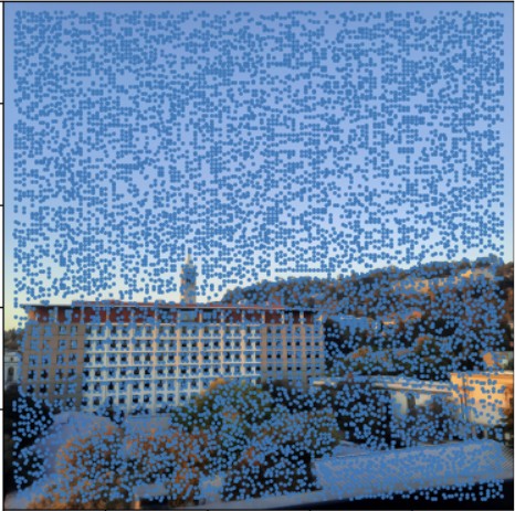
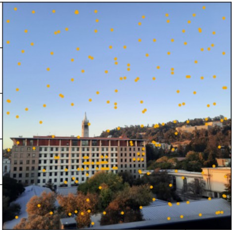
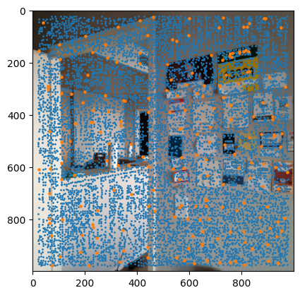
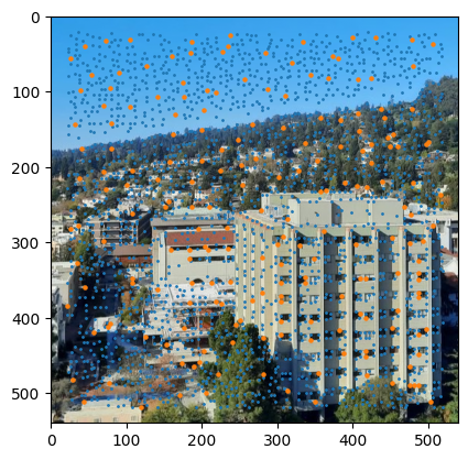
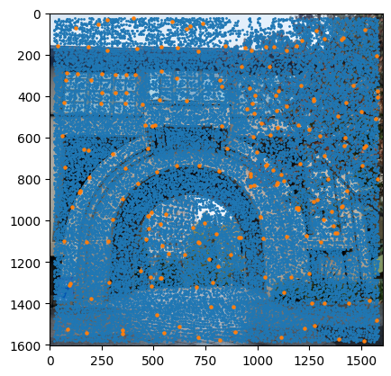
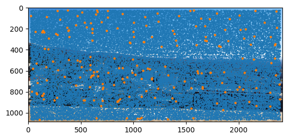
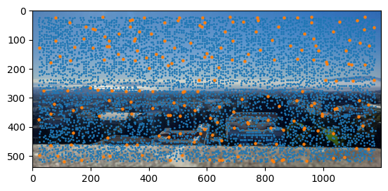
As an interesting failure case for if you don't specify enough corners, consider the following outcome when num_corners=50.

Extracting Feature Descriptors
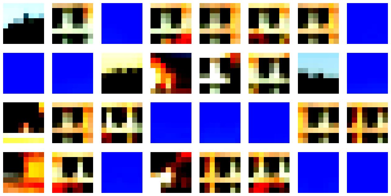
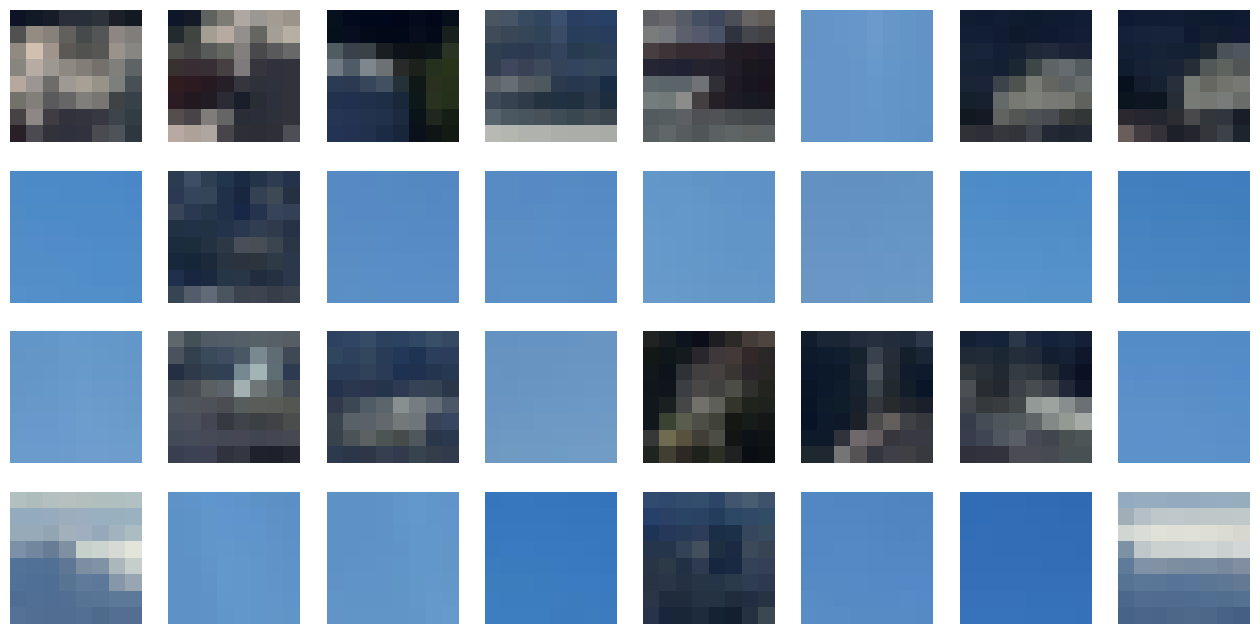
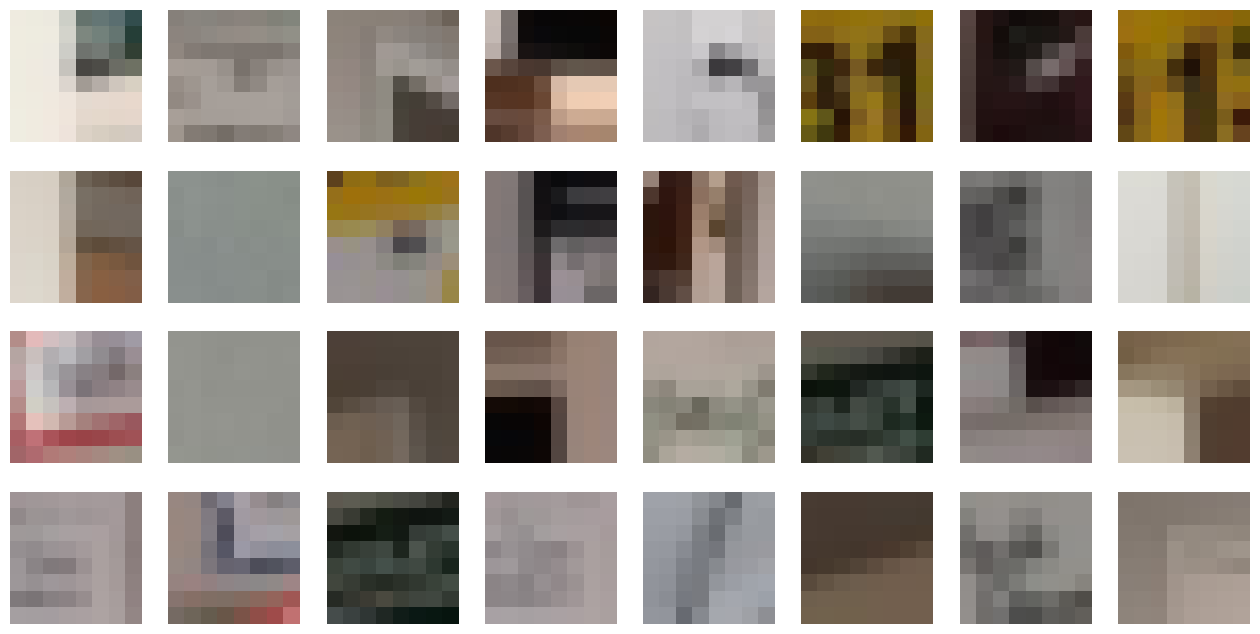
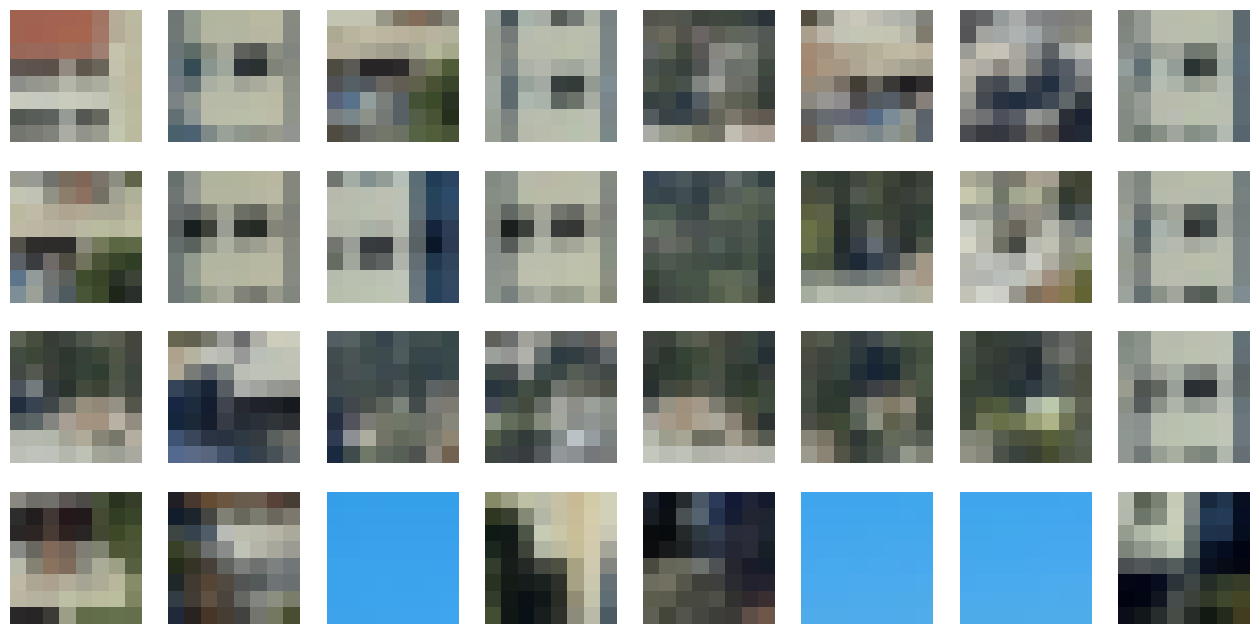
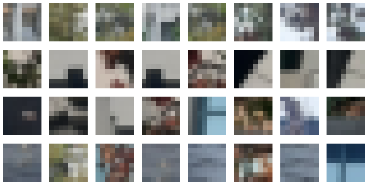
I implemented a series of functions to extract and process image features around detected corner points. The process begins with extract_patch(image, point, patch_size=40), which extracts a 40x40 pixel square centered on each corner point. It carefully handles edge cases by skipping corners too close to image boundaries.
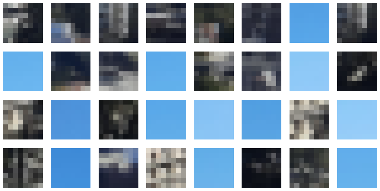
These patches then undergo two transformations. First, downsample_patch(patch) reduces each patch to 20% of its original size using scikit-image's rescaling function with channel_axis=2. Then, normalize_patch(patch) standardizes the patch by subtracting its mean and dividing by its standard deviation, making features more robust to lighting variations.
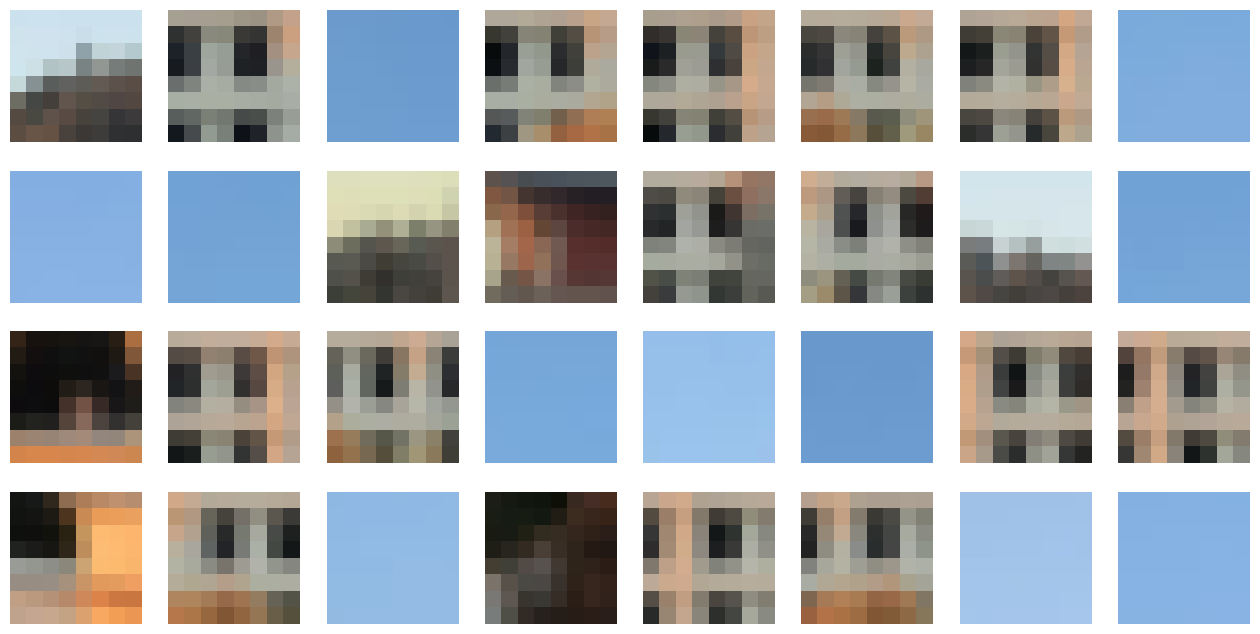
Finally, extract_features(image, corners) ties everything together, processing each corner point through this pipeline. It maintains lists of both the original downsampled features and their normalized versions, while also tracking which corner points produced valid patches. This comprehensive approach ensures we have reliable feature descriptors for matching across images. Below I show both the unnormalized features (easier to understand and display) and the normalized features.
Matching Feature Descriptors
To match features between images, I implemented a function that computes the Sum of Squared Differences (SSD) between all possible feature pairs. For each feature in the first image, it finds its two closest matches in the second image. Following Lowe's ratio test, I only keep matches where the best match is significantly better than the second-best (controlled by the ratio threshold of 0.3). This helps eliminate ambiguous matches, returning only the most reliable feature correspondences between the two images.
Pay attention to the red point in the top left corner of the Social Sciences Bldg picture, and the point near Mt. Tamalpais in the bayview picture. We shall revisit them after RANSAC to see if they made the cut.


RANdom Sample Consensus (RANSAC)
Points that fall within a 5-pixel threshold of their expected positions are considered inliers - these are matches that are geometrically consistent with the current homography. If the current iteration finds more inliers than any previous attempt, I update my "best" homography and save the mask identifying these inlier points. This approach ensures that outliers (incorrect matches) don't influence the final transformation, as they're unlikely to consistently agree with the correct geometric relationship between the images.
Finally, once I've identified the set of inlier points that yield the best consensus, I refine the homography by recomputing it using all inlier points rather than just the initial four. This refinement step produces a more accurate transformation that captures the true geometric relationship between the images.
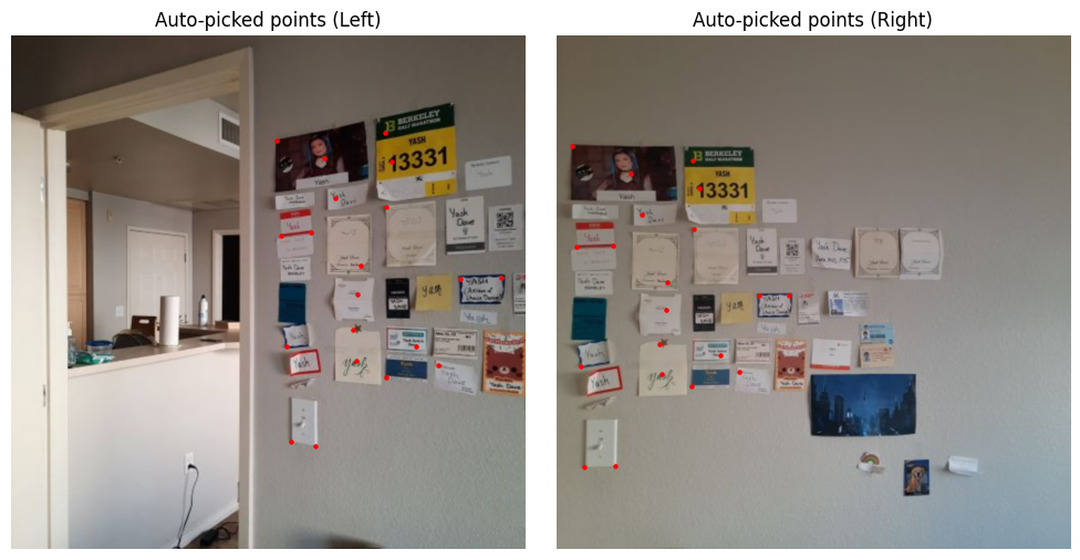
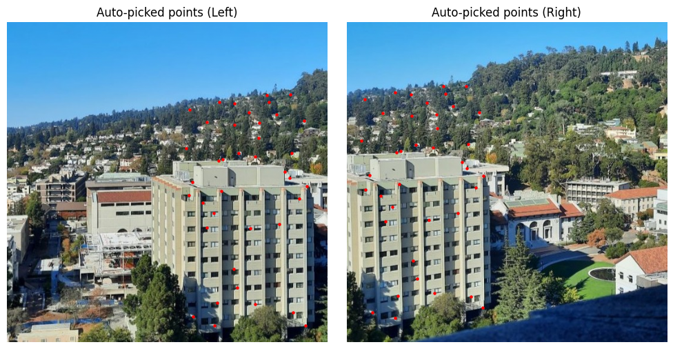
As you can see below, the red point in the top left portion of the picture in the Matched Features section is no longer present after RANSAC. While the "edges" within the sky look similar, because they are not consistent with the all the other correspondences, they are not included.

You can note that the point at Mt. Tamalpais was also excluded after RANSAC. I have also included the matched features after RANSAC for the other mosaics created, which you could expect to be slightly different to matched features before RANSAC:

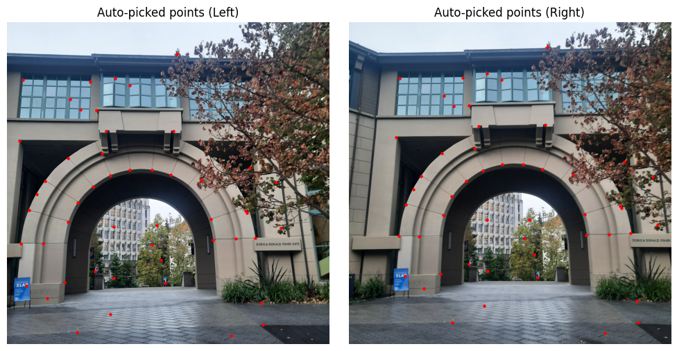

Autostitching Mosaics
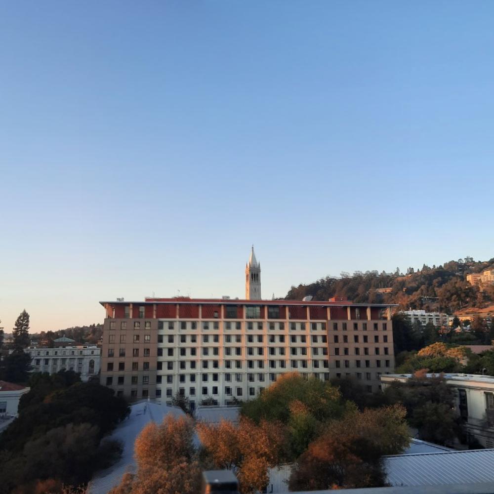
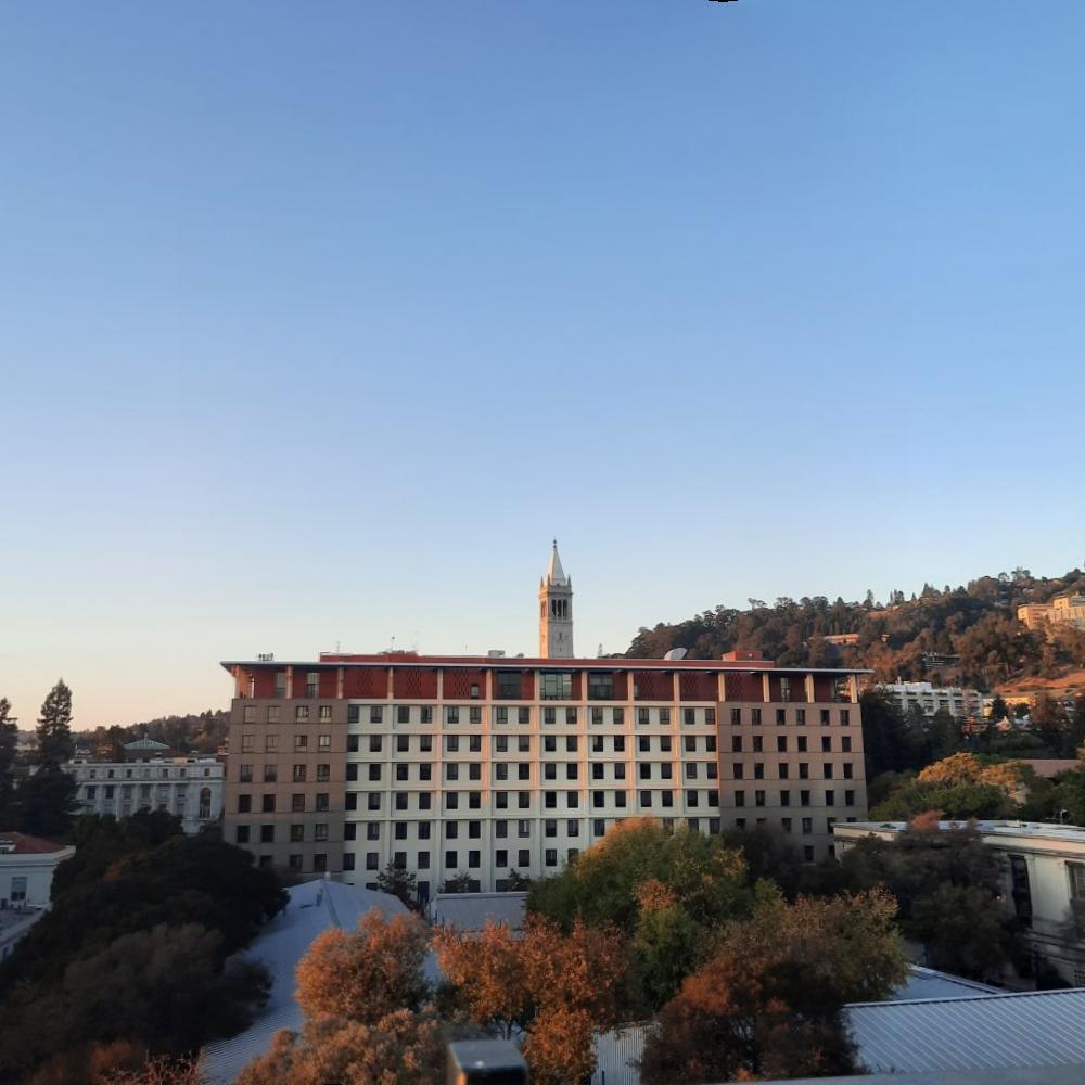
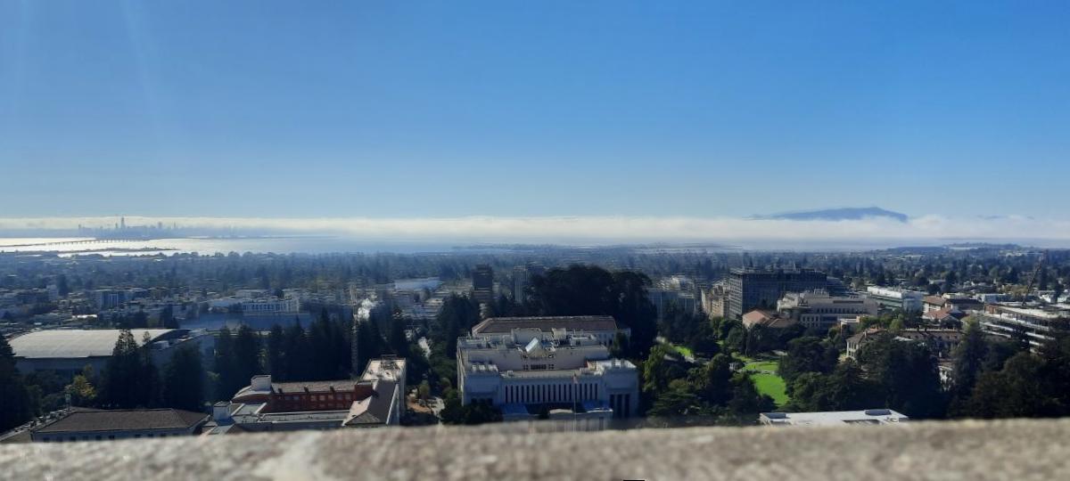
This part was simple given that all the setup was done in Part A. Now that we automatically obtain a reliable set of correspondences between two images, we can once again find the center points, compute the homography that warps the images accordingly and then blend them. I did not use the homography returned by RANSAC since I was combining them in this particular fashion.
I was pleasantly surprised with the results. The pictures were less blurry than when I manually did the correspondences, likely because I could not be as precise with the pixels. This is particularly evident with the wall picture, where the writing isn't as blurred as before. This also provided further confirmation that additional blending would not have helped because I was simply limited by the manual correspondences. Moreover, there were simply more correspondences automatically found (especially prevalent in the wall, northside pictures) than I found and that made the results more reliable.

Reflections
In terms of cool things I learned, I realised I am bad at manually doing correspondences. Automatically stitching images was ultimately (1) more efficient in terms of time (2) but also better quality on average. The process of extracting features was also super cool as it sort of felt like a precursor to all the more complicated stuff that comes with CNNs and learned filters.
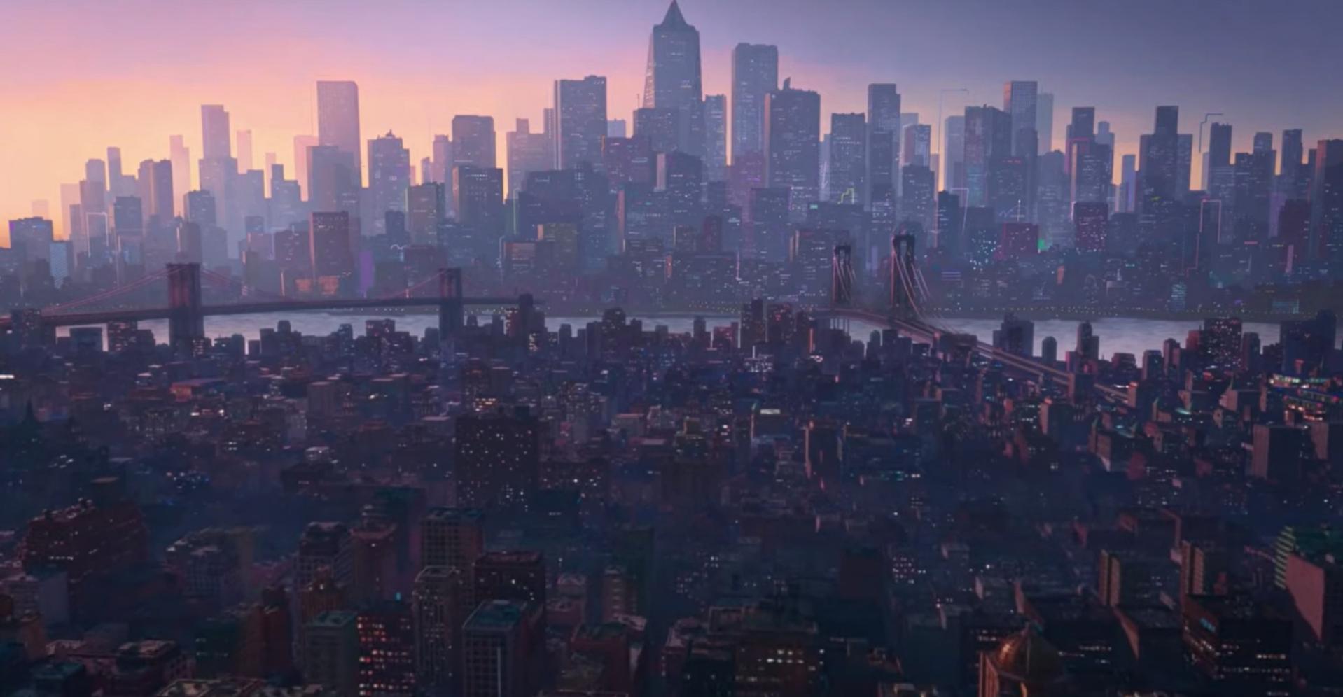
I'm also inspired to try cool new types of panoramas. I recently rewatched Spiderman: Across the Spiderverse recently, and the second I saw this shot I saw there was scope to do something. While the manual correspondences were possible, doing it automatically just felt so much cooler. Fun bonus result below, using screenshots from the movie:

